Brandon Dube for opticallimits.com under exclusive license

After the theory it's now time for a discussion of a lens. Figure 10 is an example of a real lens, and a 50mm f/1.4 design at that.  Its patent may be found on page 335 of Modern Lens Design by Smith.

Please click on the image to enlarge it!

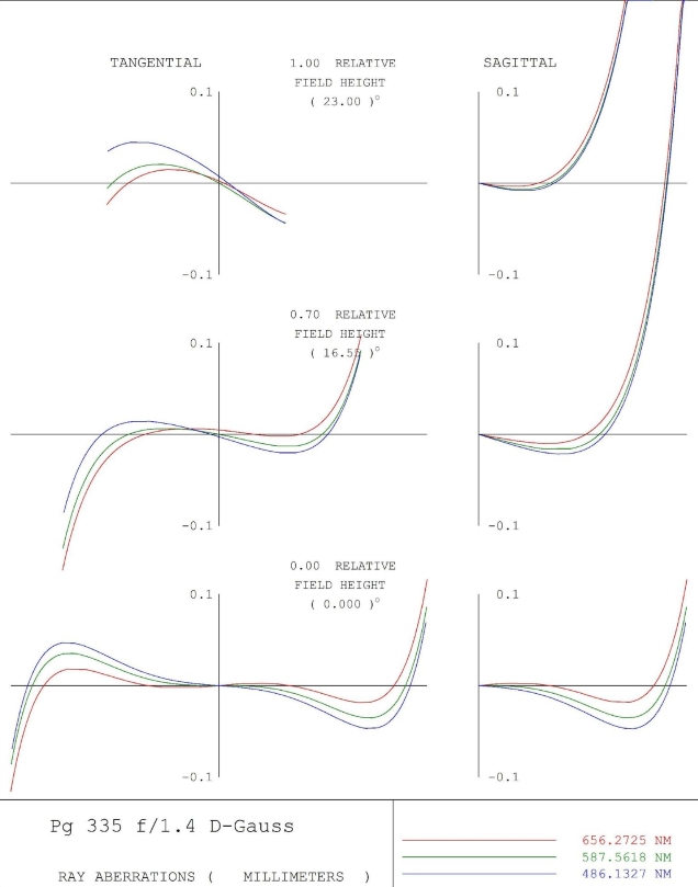Figure 10 - 50mm f/1.4 RIM Plot for Full-Frame Double Gauss Lens

The plot looks messy but honestly this is not too unusual for a fast 50mm.  I will break the plot down into its constituents for all field positions:

On-Axis (0.000°)

• 3rd order spherical (moderate, negative)
• 5th order spherical (moderate, positive)
• Spherochromatism (moderate)

7/10 field (16.55°)

• 3rd order Spherical
• 5th order Spherical
• Spherochromatism (small)
• Petzval (moderate)
• Coma (small)
• Astigmatism (small)
• Sagittal Oblique Spherical (very large)

Full field (23.00°)

• 3rd order Spherical (moderate, negative)
• 5th order Spherical (moderate, positive)
• Spherochromatism (small)
• Petzval (moderate)
• Coma (moderate)
• Astigmatism (moderate)
• Sagittal Oblique Spherical (enormous)

At full field, the plot’s shape is almost entirely driven by the Petzval and stacked coma and spherical merely modulate it. You may also see that the plot is cut off for the 7/10 and full field positions.  This is one way to see vignetting – it is apparent that a bit more than 50% of the light is cut off at full field, or a bit more than 1 stop of vignetting.  One can see that the rays are headed in a very poor direction and would be very, very badly corrected if the vignetting wasn’t present.  In this way, vignetting is a valuable correction technique and may be arbitrary provided physical constraints are not present and/or the design criteria are flexible with regard to peripheral illumination.  The distortion is entirely missing from the RIM plot, and Petzval and astigmatism are hard to discern unless they are the biggest issue.  

By now you may also wonder what this lens looks like - figures 11 and 12 show the lens and what the field curves (astigmatism, Petzval, distortion) look like.

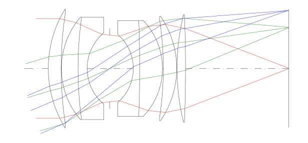Figure 11 - Lens Diagram for the 50mm lens

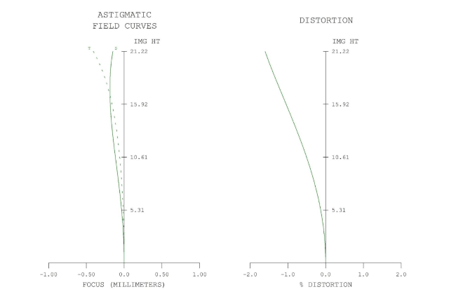Figure 12 - Field Curves for the 50mm f/1.4 lens

In the lens diagram vignetting may also be seen.  The “notches” in the center of the lens are the aperture stop.  If it is filled by the rays, there is no vignetting.  The blue full-field traces clearly do not fill the stop, so it can be seen that the lens is vignetted.  From the field curves it is evident that distortion is reasonably well controlled, and that the lens’ field curvature is decently small, as is the astigmatism.  

I will point out at this time that the coma in this lens is small and is not the dominant aberration.  It is all the rage these days when a new lens is released to check fi it has “coma” by shooting a star field and looking at what the stars look like in the corner of the picture.  This is a rather harsh torture test for a lens, since the typically strongly clipped stars present an enormous object-space contrast.  The dominant aberration in this lens is oblique spherical by a factor of more than two.  Figure 13 shows a spot diagram for the lens.  The full field spot may look familiar, it is the internet-famous “wings” - what many review websites label incorrectly as “coma.”

Please click on the image to enlarge it!

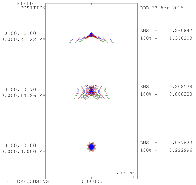Figure 13 - Spot diagram for the 50mm f/1.4 lens

How “fat” the wings are is a good measure for how out of focus the sagittal plane is, while their “width” or length is a measure of how much oblique spherical is present.  In the spot diagram the coma is actually mostly invisible because of how much larger the oblique spherical is.  In the very center of the full-field plot you see the blur tend towards a “comet” shape – this is coma.  Figure 14 is the lens' MTF, something photographers are maybe more familiar with.

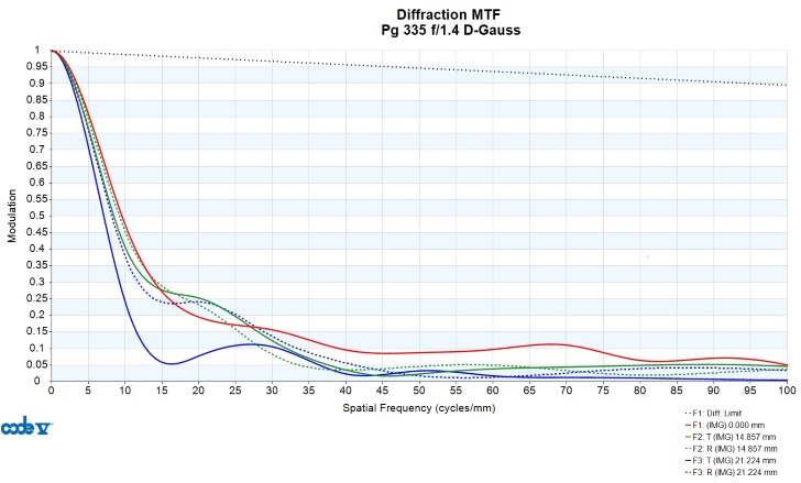Figure 14 - MTF for the 50mm f/1.4 lens

These curves extend to high spatial frequencies – perhaps a method for a bare bones analysis is necessary.  Lenses may be said to “outresolve” the sensor if the MTF is greater than 50% at the (compensated) Nyquist frequency of the sensor.  The Nyquist frequency is simply the max spatial frequency which can be recorded i.e.

The factor of one half is due to the fact that to record a line pair or complete cycle (white-to-black) two samples are needed.  A compensation must be done after that to adjust for the sensor’s own degradations. The Bayer pattern immediately means that of it takes a 2x2 chunk of data to get full color for a single pixel, so we may throw away 50% of what is left. On top of that, if an optical low pass filter (OLPF, anti-aliasing filter) is installed we may take off another 15%.  For e.g. the Canon 5Ds we have:

This is roughly comparable to something like a 7D mark II or a Nikon D7200.  Lower pixel density sensors e.g. a Sony A7 mark II amount to more like 35lp/mm or so.  It should be noted that the resolution limit of the sensor is not linear with increased pixel count; as the pixels are shrunk there is some inevitable loss on the sensor’s side of things, so the OLPF adjustment should be increased as pixel density rises.  For the 5Ds I may use a value closer to 30%, but things are further complicated because this effect is stronger towards the edges (for those interested, this is mostly due to how light is refracted at flat surfaces and is remedied by telecentric lens designs).  

From the sensor analysis it is clear that the lens is not up to the task of “outresolving” typical cameras wide open.  The specifics are outside the scope of this article but through optimization lenses can be improved beyond their starting performance.  Most lenses are actually not original designs, but an older lens by the same firm or a patent which has been modified and optimized to fit the needs of the lens being designed.  In this case, by adjusting the lens shapes and aspherizing the rear surface the performance was easily brought to a level somewhere between that of “last generation” fast 50mms and the current generation (e.g. sigma 50A, Zeiss Otus, SonyZeiss 55/1.8, and so on).  The oblique spherical (wings) remains a problem, but the MTF is good enough for a sharp center wide open on your typical full-frame sensor.  It is below in figure 15.  Figure 16 is the optimized lens’ RIM plots.  Figure 17 is the spot diagram, to help correlate the RIM plot to what the image from the lens looks like for many field positions.  Except for MTF, I am now using 6 field points.  3 are sufficient with an all-spherical system because local maxima will appear at √2 (.7) and the extreme field tells the corner performance.  Thus, if any field point other than full field is the worst, it is 7/10.  With an asphere the situation becomes far more complex and it is necessary to use more field points.  The more complex the system of non-spherical surfaces, the more field points should be used to ensure there is no especially good or bad point in the image field.  Only three points are used for MTF to keep the graph from becoming overly dense.  

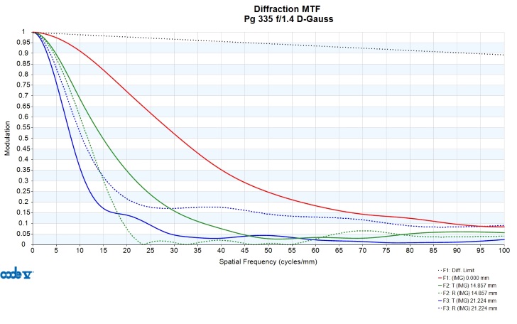Figure 15 - The same 50mm f/1.4 lens after ten minutes of optimization

Please click on the images to enlarge them!

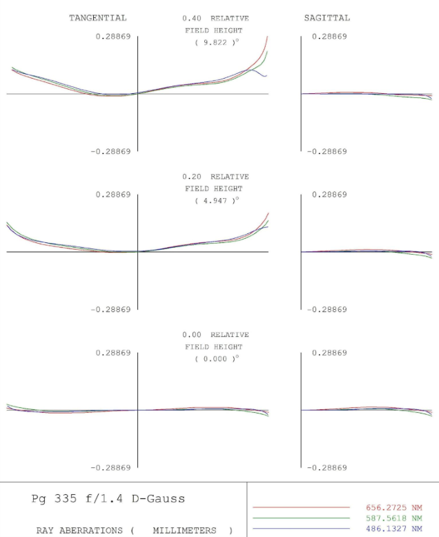Figure 16.1 - RIM plots for 0, 2/10, and 4/10 field for the optimized 50mm lens

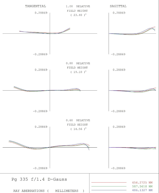Figure 16.2 - RIM plots for 6/10, 8/10, 10/10 field for the optimized 50mm lens

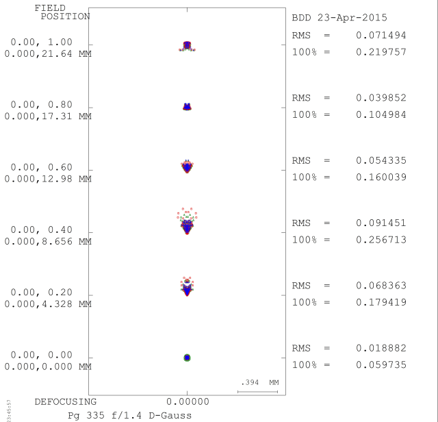Figure 17 - Spot Diagram for the optimized 50mm f/1.4 lens

In this version the lens has a flat tangential field but a “badly” curved sagittal field.  This astigmatism is still smaller than the previous version, but it is the biggest limitation aside from the high coma in the middle of the image, which can be corrected with more optimization (though the lens will walk fairly far away from this solution).  The new rendition has a larger rear element, but it is still smaller than the throat diameter for any popular camera mount, so vignetting could still be reduced. Due to the greater element size and inclusion of an aspherical surface, cost would be a significant factor to look at.  Unfortunately the lens would not improve too rapidly as it is stopped down, since the RIM plots are fairly flat due to a particularly even contribution from 3rd and 5th order spherical aberration.   Note the difference in spot size – the original lens had a max rms spot size of 260 microns (almost 50px) while the new one has a max rms spot size of 90µm and a mean of closer to 10µm, which is about 2px on most APS-C and Full-Frame sensors at this point (though I don’t know for how much longer that will be true) and all that is needed for a “tack” sharp image.  Within the lens design community, it is commonly said that a spot size on the order of magnitude of the pixel size is good, this optimized lens meets that description.

A useful metric for potential lens resolution may be in terms of megapixels derived from the diffraction limit, so a comparison of different f numbers versus the number of megapixels on a full-format detector is below in table 3.  Please note that several assumptions are made and the chart should not be taken as gospel.  The wavelength is fixed at .5876µm as for the chart on the aberrations theory page, then the spatial frequency at which MTF is 50% is multiplied by the detector dimensions and a factor of 2 along each side to convert cycles (2px) to a pixel dimension.  This is based on the assumption that MTF 50% is the limit for distinguishable features, sharpening and deconvolution will enable lower resolution lenses to appear as good as this number.  The assumption is also made that the sensor’s MTF at its nyquist frequency is 100% which is never the case.  This is merely the highest resolution the lenses, not the system, support.  

Table 3 - Maximum megapixel count supported by various f numbers

I have shown MTF out to 100lp/mm to give a better sense of comparison relative to the diffraction limit, despite the lens performing badly over a very large portion of that spatial frequency range.  Photographic lenses typically are not diffraction limited due to the many constraints placed on their design (e.g. maximum length, maximum diameter, weight, necessity for internal focusing, inclusion of an image stabilization unit, minimum back focal length, cost, etc) and plain lack of necessity for lenses of such high resolution.  Particularly well corrected telephoto lenses such as Canon’s 300mm f/2.8L II and 400mm f/2.8L II or Zeiss’ 135mm f/2 APO-Sonnar or Nikon’s 200mm f/2G II are closer than the overwhelming majority of lenses which you can purchase for your camera today.  To give a sense of the performance of a lens of this class, figure 18 has been produced with data graciously provided by Roger Cicala of LensRentals.com.  Five lenses were tested for MTF under the standard Lensrentals procedure, and the best lens was tested out to 100lp/mm.  MTF measurements were done on a Trioptics ImageMaster MTF Bench and analyzed in order to produce the figure.

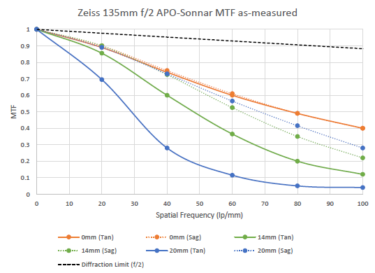Figure 18 - MTF of the Zeiss 135mm f/2 APO-Sonnar lens

In the case of this 135mm lens, we may observe a drop in the resolution towards the edge, but mostly for the tangential image plane.  This, likely indicates that the lens suffers from astigmatism.  Astigmatism in lens design is thought of as a difference in the field curvature (Petzval) for the sagittal and tangential planes.  Here it appears that the sagittal plane is quite flat, and the tangential plane is curved such that the edges do not fall to the same focus as the center.  Referencing the manufacture MTF curves, available here for f/2 it is apparent that one of two situations is the case; either the curves are generated by mounting a sample lens to an MTF bench such as the ImageMaster used to produce this data or an Optikos LensCheck bench and the results are from the medial focus or focal plane of least astigmatism, or Zeiss compensates for field curvatures to produce their MTF curves.

So where do we stand?  If you have read this far, you have a small glimpse into the world of lens design and optimization.  With this, you can see lenses the way designers often see them – in terms of RIM plots and MTF curves (albeit in a different format to manufactures’ published-for-consumer curves).  Likewise, you have a basis for understanding resolution limits and the implications of higher resolution sensors and can see that lenses can, as a limit, outpace sensors for a long time to come.  Cost size and weight must increase for better resolution, but this is somewhat expected.  I might also point out that the system for this “simple” 50mm f/1.4 lens totals about 45 variables to optimize – not an easy problem.  Luckily, CAD software will run the math for us, and help lead to solutions which are ultimately far beyond the limits of what was possible previously.  

Watch out for the next article in the coming months which will cover historical design forms such as the double-gauss, retrofocus, tessar, sonnar, telephoto, and so on.  We will be looking at many more RIM plots if you continue reading ☺