Alternative colorimetric systems and color models

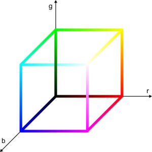
When using the colorimetric systems discussed so far (CIE-XYZ) and the color spaces defined within it, one can identify a color by its coordinates (or in other words by the amounts of each primary that need to be mixed, additively or subtractively, to obtain that particular color). Though far from being accurate, the color cube below (of which only the edges were drawn – the cube is actually solid) gives a representation of a three- dimensional rgb color space.

Other ways of identifying a color can be devised that do not use primary colors to describe the reference color space. But since the visible colors are fundamentally the same, these alternative color spaces are in fact mathematical transformations of the CIEXYZ. Again, they are a different means of describing the same thing. They were created out of the need of relating color descriptions to human perception. In this respect CIEXYZ is far from being intuitive. When was the last time when you looked in the distance at sunset and remarked: ‘Oh the sky looks wonderful! I sure like colors with x and y values around 0.4…'?

For instance, the essential properties of colors are suitable as color coordinates for an alternative system.

HSL and HSV – the non-identical twins of color models

In this respect, he HSL (Hue, Saturation, Luminance, or, somewhat incorrectly, Luminosity) and HSV (Hue, Saturation, Value) color models are very similar. These are both three-dimensional spaces employing the ‘hue wheel' as a common element. This hue wheel or disk has as its border a circle containing all the pure colors (or hues) of the CIE chromaticity diagram.

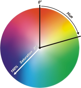
Hue is described by the angle on this circle, with zero (and 360) degrees corresponding to pure red, as in the rough representation below.

Saturation is described by the distance from the center of the circle, which by definition has zero saturation. The colors of maximum saturations are on the circle bordering the hues disk.

In the HSV (also called HSB, B for brightness) color system, the colors of maximum saturation (on the edge of the hue disk) are not necessarily pure (spectral colors). The HSV is an alternate representation of a given RGB color space, and the saturated colors in HSV are in fact the colors bordering the corresponding RGB triangle in the chromaticity diagram. For this reason, the HSV color system is said to be device dependent, meaning that it is not an absolute colorimetric space, but relative to the gamut of the RGB color space it describes. The third coordinate in HSV (or HSB) is the value or brightness; black has zero brightness. Starting from the hues disk one can imagine the HSV space as a collection of hues circles with varying color value, one on top of the other and of the same size (creating a cylinder) or of sizes diminishing with value (a cone).

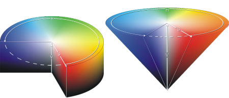
Images reproduced under GNU public license

While a cone is more intuitive, as all colors converge to black for zero value, the cylinder shape is more correct as a mathematical representation.

As a method of describing colors, HSV is particularly useful when creating what are called color progressions, meaning, in a restricted sense palettes of related colors having the same or related hues, saturations or values. In this case, knowing the actual figures for the red, green and blue primaries is simply not necessary and HSV offers a more intuitive representation of the relationship between colors. But the thing to be remembered is that HSV is just mapping a particular RGB color space; it is a different coordinate system describing not more and not less than the original RGB space.

The HSL, also named HLS and HIS (I for intensity, which is the same as lightness) is a similar representation to HSV, in that they are both nonlinear transformations (alternative mapping systems) of a particular RGB color space (this fact making them relative and not absolute ways of measuring color). The other similarity is that they both employ the hues wheel. And this is the point where the two representations diverge. Good representations of HSL are a sphere or a double cone. In the HSV cone, the number of colors decreased with value. In the HSL cone, they still do, but the maximum is not for maximum lightness but for 50%. While HSV has a large number of colors with maximum value, HSL only has one: white.

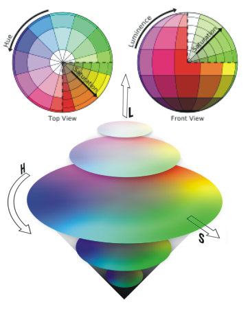
Images reproduced under GNU public license

Both HSL and HSV are more intuitive ways of representing the RGB color space. It is debatable which of the two represents a description of color more suitable to humans, but HSL seems more adequate due to the fact that it creates truly independent representations for saturation and lightness. In HSV 100% lightness corresponds, among others to very saturated colors making it unnatural to think about, say, bright red as a very light color, which is not the case in HSL. On the other hand, HSL describes a lot of very light colors as fully saturated, which again contradicts the way we normally refer to color, making HSV a better system in this respect.

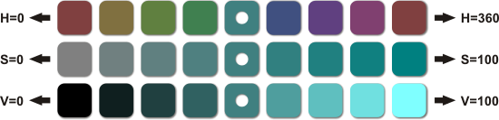
The two figures below illustrate the concepts introduced in this section. The first one refers to HSL and the second one to HSV. The perforated patch will be our reference and it represents the color with 50% of everything (180 degrees of hue shift, and a saturation of 50 and a lightness or value respectively again of 50).

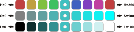
One thing you notice right away is that the reference color in HSV is different from the one in HSL. This is precisely because the two spaces have a different way of defining the brightness (and to some extent saturation) and the same number for value and lightness yields different results. The third row of each diagram perfectly illustrates the difference between the concepts of value and lightness (V=100 results in a bright shade of, in this case 50% saturated cyan; L=100 is white).

The second rows (saturation) also show a difference between the two systems. In HSL, increasing saturation results in increased perceived brightness. In HSV, as mentioned before, this does not happen. Hue is common for both systems but the colors on the first row of each diagram differ in brightness (as expected). And of course the first and last colors are identical, as 0 and 360 degrees are precisely the same thing.

To prove the point even further, the following figure shows the effects of changing the hue, saturation and lightness of all the colors of an image.

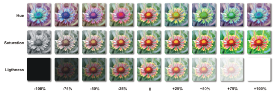
These are the results you get when you manipulate a picture in your favorite image editing software. Starting from a reference picture (the one in the middle on all three rows), each row shows the effect of modifying only one of the H, S or L components (again – of the whole image) in roughly +/- 25% steps.

Lab – the mother of all color manipulation

The notation Lab in graphics software almost always represents the CIELAB color space. In this text, Lab will be also used in reference to CIELAB.

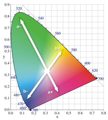
Lab is derived from the chromaticity (horseshoe) diagram by first changing the x and y axes to a and b, like in the diagram below. A negative a (or a*) value indicates a greenish hue while a positive a means a magenta/reddish one. On the b (b*) axis, negative values stand for blue and positive for yellow. A value of 0 for L* is equivalent to black and L* = 100 describes white.

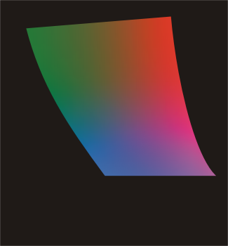
Now due to the shape of the horseshoe diagram, which considering the new a and b axes is not rectangular, a slice of CIELAB in the ab plane for a given L is not rectangular. This means there are values of a and b for which no real color exists. For different values of L, the representation in the ab plane changes. The figure below shows a slice in the CIELAB color space for L=65.

As a quick reminder, CIELAB and CIEXYZ are 3D spaces and, as mentioned before, in simple on-screen representations, only a cross section is shown. More importantly, CIELAB and CIEXYZ are far wider than the gamut of any presentation medium, thus the illustrations that refer to these color spaces are never exact representations, but merely helpful visualization tools.

Just as HSV and HSL, Lab is another form of representing the space of colors visible to humans. The relationship between colors in CIELAB is relative to the white point that is being used. If the reference white point is always kept the same, it becomes an absolute (device independent) space.

Theoretical aspects being covered, we now come to the practical side of Lab. Its greatest advantage as a tool for representing and characterizing color over CIEXYZ is its greater uniformity; colors values on the three axes are distributed more closely and more linearly with respect to the human perception of color. In RAW processing applications (using Lab), users are able to change the white balance (essentially the white point of the color space) and the blue/yellow and green/magenta distribution of colors within the image (shifting every color present in the picture proportionately on one of – or both – a and b axes). The CIEXYZ diagram is not appropriate for showing an example of this because of its being highly non- linear and quite deceiving in the representation of color distance.

Moreover, by ‘having the ability' to be an absolute color space and wider than any device-dependent space, Lab is ideal as an intermediary step when changing between two spaces. The next section deals with color management and changing between color spaces.

Similar to what we did with the other color systems, the following example shows the influence of changing only one of the three color components in Lab, from minimum to maximum, in roughly 12.5% steps.

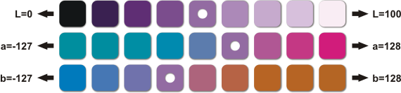
The mauve perforated patch is our reference color. L=0 gives black and L=100 white. As stated, changing the value of a makes the color greener or more magenta and the value of b gives the color a blue or yellow- orange tint.